
Basic Statistics
Many people get intimidated by statistics, but just remember that the majority of your data analysis will probably only require simple math that you learned in fifth grade. If you need to do more advanced statistics, such as hypothesis testing, you may want to seek the help of a statistician.
You can also refer to our advanced analysis section to learn more about statistical tests. But there is a lot you can do on your own that you likely do not even realize!
There are several types of descriptive statistical analysis that anyone can do:
Descriptive Statistics
Each of the three main categories listed under the Project Design section are what we call descriptive statistics.
You may be thinking, “Why do I care about trying to describe my data? I just want it to give me answers!” Well, descriptive statistics will often give you answers, and they will often help you understand your data better and make your answers more meaningful. Whenever you do a statistical analysis project, you should start by running some basic descriptive statistics.
Let’s say, for instance, you are doing a study on childhood weight. You collected weights from several different children. Here are the different weights you found:
13 36 98 77 42 50
110 22 49 81 26 38
OK, now tell me about your data. Can you describe it to me? Can you tell me anything interesting about the data? I will bet you cannot right now, but as you study the topics in this section, you should be able to soon.
Counts
Let’s use some sample data from a study on childhood weight. Weights from several different children were collected. Here are the different weights in the dataset:
13 36 98 77 42 50
110 22 49 81 26 38
How Many?
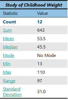
The first descriptive statistic you should know is a count. This is just as simple as it sounds; it is a count of how many items or “observations” you have. If you count how many child weights there are above, you would find that there are 12.
Sometimes in statistics we call this the “n”, indicated by a small letter n. So here our n=12.
Count (n) = 12
Why do I need to use a count?
Big deal, you are thinking. Who cares about a count? Well, this number gets used a lot in statistics. It is important to know how many observations your dataset contains for you to evaluate your results.
For instance, if this were a real study being done and you were trying to make a conclusion about childhood weights, would you really trust a study that only had 12 children in it? Obviously, we would need to have more observations to make valid conclusions. But for learning purposes, 12 is a great number to work with.
Sums
A “sum” is the sum of all the data (the observations) in a dataset. Once again, we are using quite simple math here. Just add up all the numbers below from a dataset of childhood weights (you can use a calculator if you prefer).
13 36 98 77 42 50
110 22 49 81 26 38
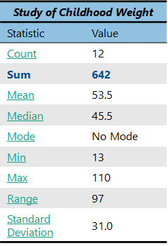
Sum = 13+36+98+77+42+50+110+22+49+81+26+38
The answer is 642. Should this number mean anything to you right now? Not really. It is good to have, but it will only become useful later when you use it in other statistical analyses.
Measures of Center: Mean, Median, and Mode
Measures of center are some of the most important descriptive statistics you can get.
In our society, we always want to know the “average” of everything: the average age, average number, average speed, etc. etc. It helps give us an idea of what the “most” common, normal, or representative answers might be. Essentially, by getting an average, what you are really doing is calculating the “middle” of any group of observations. There are three measures of center that are most often used:
- mean
- median
- and mode.
Mean
Finding an average is often called the “mean.” The mean is the most commonly used measure of center.
So, let’s find the mean of a given dataset. Here is a sample dataset of child weights:
13 36 98 77 42 50
110 22 49 81 26 38
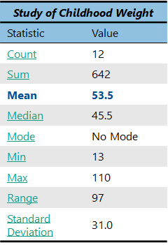
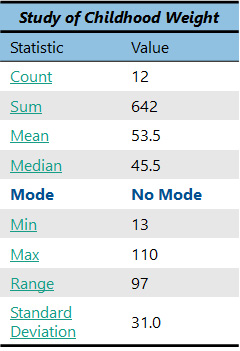
How do we find the mean? All we do is take the sum of the observations and divide by the count. “Wow,” you’re thinking. “I just happen to already have the sum and the count of these numbers” (see chart on right). Good for you! Now you get to use them both.
Just take the sum, which is 642, and divide it by the count, which is 12. The answer is 53.5. So, we now know that the average (or mean) weight of the children in our study is 53.5!
So, what does this mean? Well, it depends on your study. Maybe you expected that the average weight of the children would be smaller for some reason, so the mean alone is an interesting finding to you. Or maybe you were comparing this group of children with another group of children and found that the other group had an average weight of 84. You would conclude that the other group consisted of much heavier children. Very often, you will find that individual statistics do not mean much on their own, but they take on important meanings when you compare them with others.
Median
Another important measure of center is the median.
The median is the middle observation in a set of data. Let’s calculate the median for a sample dataset on childhood weight.
13 36 98 77 42 50
110 22 49 81 26 38
Calculating the Median
In the dataset above, what is the middle observation? Well, before we can figure this out, we must properly order the observations in a logical manner to ensure they make sense. We will order them from smallest to largest, as shown below:
13 22 26 36 38 42
49 50 77 81 98 110
Odd Number of Observations
In a dataset that has an odd number of observations, this is extremely easy; it is simply the number smack in the middle (the one with an equal number of observations above and below).
Even Number of Observations
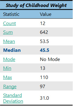
However, in our case we have 12 observations, which is an even number. This means that we need to take the two observations in the center and average them. In this case, the two observations in the middle are 42 and 49. When we take the average of these two numbers (remember, to do an average, you sum the two numbers (42+49 = 91) and divide that number by the count, which in this case is 2), we get 45.5. So, our median is 45.5.
What Does the Median Tell Us
So, what does the median mean? Well, like the mean, it provides a helpful measure of center of our dataset. We now know that the median weight of the children in our group is 45.5. But it is also helpful to compare the median with the mean. 45.5 is obviously less than the mean, which was 53.5. Often, the mean and median will be the same in a dataset, but sometimes they are different, such as in our case. When the mean and the median are the same, you know that the dataset is “normally distributed.” When the mean and the median are different, you know that the data are “skewed” in some way.
What do I mean by skewed? Well, unlike the mean, which was a mathematical calculation using every observation in the dataset, the median ignores what the numbers say and just uses the middle observation. Which one is right? They both are. Neither one is necessarily better than the other. So why use a median? Well, there are certain kinds of data where you will be concerned about skewing. Skewing is when the mean is pulled higher or lower than the median because of very high or very low values.
Let’s say, for instance, you wanted to know the typical income of all the people you know. First, you would collect the data. You would probably get a wide range of answers, with most of them being between $20,000 and $150,000 a year or so. However, we can imagine that you may know some people who make millions and millions of dollars a year. If you include even just one or two of those people in your dataset, the entire dataset would be skewed.
Your dataset look might like this:
$20,000 $25,000 $35,000 $37,000
$42,000 $45,000 $58,000 $69,000
$80,000 $110,000 $140,000 $250,000,000
Notice how 11 out of the 12 observations fall within what most would call a “normal” income range, but the last person makes a lot more money.
If you were going to take a median of the above data you would get $51,500. But if you were to calculate the mean (the average), it would be a whopping $20,888,000! Talk about skewed data. Would you really want to go around telling people that the average income of people you know is more that 20 million dollars a year? People would think you’re crazy, but you would actually be telling the truth. That is the real mean; however, the median would more accurately represent the income of “most” of the people in this example.
Should I Use the Mean or the Median?
So, because what we really want to know is how much money “most” people make, sometimes we have to control for those situations where a few observations can seriously distort our mean. In this case, we would decide it best to report the median income rather than the mean.
Hospital length of stay is another example of data that is often skewed. Most people stay only a few days when they are admitted to the hospital, but there are a few people who have hospital stays of more than 365 days or longer who significantly skew the data. In this case, you also would probably want to ignore the mean and just report the median. In general, however, most people expect you to report the mean unless you have a good reason for not doing so.
Mode
The third measure of center is the mode. This one is easy; the mode is simply the most frequent observation.
For example, let’s suppose that in a dataset of child weights, there were actually two children who were 50 pounds (and all the other weights were still just listed once). Then 50 would be the mode of our data, because 50 was the most frequent observation. Let’s also assume that in addition to those two 50 pounders, there were also three children who were 77 pounds. Now what would the mode be? Yep, it would be 77, because 77 is now the most frequent observation.
13 22 26 38 36 42
50 50 77 77 77 110
(Modified dataset of child weights.)
As you can see, this measure of center hardly requires any math at all. In the dataset of child weights, we have been using (see below), there are no repeating observations at all, so we would say there is no mode.
13 22 26 36 38 42
49 50 77 81 98 110
Using the Mode
How useful is the mode for you? Usually it is not that useful. The mode is by far the least commonly used measure of center. The times when it is most useful are when you are working with open text data or categorical data, such as multiple choice.
For instance, if I asked several people in my family where they would most like to go on vacation and the most common answer was Hawaii, I would be able to effectively say that the mode was Hawaii, and I should probably not plan my next trip to Milwaukee.
However, if I were presenting this data to others in the real world, most people would want to see the percentage breakdown of how many people said Hawaii compared with the percentages for other top locations. This is the reason the mode is not entirely useful to you; there are usually better ways of discussing data that you get from a mode. But it is still important to understand what the mode is.
Min, Max, and Range
The min and max are also useful for understand a given set of data…
13 22 26 38 36 42
49 50 77 81 98 110
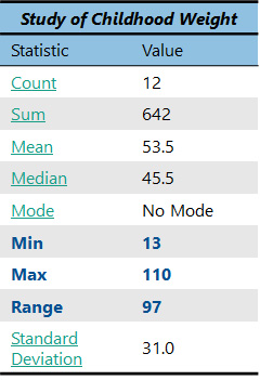
Using the dataset of child weights above, we can find the min and max. The min is simply the lowest observation, while the max is the highest observation. Obviously, it is easiest to determine the min and max if the data are ordered from lowest to highest. So, for our data, the min is 13 and the max is 110.
Using the Min and Max
Finding the min and max helps us understand the total span of our data. There are a variety of reasons you might do this depending on the study. It is usually something that is nice to know and helps you feel more familiar with your data. Or you can do a min and max to help you identify something wrong.
For instance, maybe for our study of childhood weight, we only want to focus on children over the age of two years old. By identifying the min of 13 pounds, we may be concerned that we have unknowingly gotten an infant in our study. We would then want to further investigate how this occurred, if there are other infants in our dataset, and what should be done with these data as we proceed with the data analyses.
Range
Sometimes it is also useful to use the min and max to calculate the range of a dataset. The range is a numerical indication of the span of our data. To calculate a range, simply subtract the min (13) from the max (110). The range for this dataset is 97.
The range is another example of something that is nice to know but is not particularly useful unless we are comparing it with something else.
Standard Deviation
The standard deviation is useful when comparing one dataset to one or more datasets.
You have probably heard of the term standard deviation before. This is one way of measuring the dispersion of a given set of data. What do I mean by dispersion? Well, if we use a sample child weight dataset (shown below), the data ranges from 13 to 110, with a mean of 53.5. It is a fairly wide spread of data.
13 22 26 38 36 42
49 50 77 81 98 110
Well, what if the data had the exact same mean, but instead ranged from 45 to 62? You would determine that this would be a much tighter range, right? There would not be as much spread or dispersion from the mean. It is important to have a good understanding of the dispersion of your data so it can be properly compared to other data. The standard deviation is one tool for assessing data dispersion.
Calculating Standard Deviation
There is a little more math involved in calculating the standard deviation, but it is not advanced. The standard deviation is simply the square root of the average squared deviation of the data from the mean. Before you allow this definition to scare you off, let’s calculate the standard deviation for the sample dataset of child weights together:
13 22 26 38 36 42
49 50 77 81 98 110
Step 1: First, we calculate the mean (or average) of the data. Fortunately, we have already done this. The mean is 53.5.
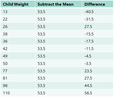
Step 2: Now, subtract the mean from every item in the set. Often, a table is helpful in performing these calculations. The calculations have been performed below:
Notice that if you were to sum all the numbers in the “Difference” column, you would get a sum of zero. This makes sense, of course, because by definition, the mean should be the exact middle value equidistant to each of the points in the dataset, so the positive and negative differences will always balance each other out. Adding these numbers will always result in zero, regardless of how condensed or dispersed the data values are about the mean.
Step 3: Square the difference between each number and the mean (the third column in the table above).
To prevent our sum of the Difference column from resulting in zero, we can square these numbers. Remember this means multiplying each number by itself (-40.5 times -40.5 equals 1640.25). The new squared differences are now as follows:
Difference Squared:
1640.25 992.25 275.25 240.25 240.25 306.25 306.25
132.25 20.25 12.25 552.25 756.25 1980.25 3192.25
Step 4: Sum the squared differences. We get a sum of 10,581.
Step 5: Divide this sum by the number of items (for a sample, you would instead divide by n-1; remember n is the count).
Since our dataset was a sample of child weights, we will divide by n-1 (12-1=11). The answer is 961.9 This number is called the variance.
Step 6: Take the square root of the variance to find the standard deviation.
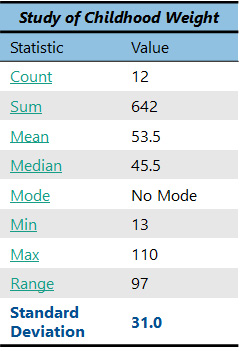
Taking a square root converts the variance from squared units to the original units of measurement. Our standard deviation is 31.0.
Yeah! We did it! Phew…
How Can We Use the Standard Deviation?
So how does this relate to the real world? Many people wonder how we know which is better: a large standard deviation or a small standard deviation, but it all depends on what you are asking. Remember, the smaller the standard deviation, the more closely the data cluster about the mean. This information is useful in comparison to other datasets.
In the sample child weight dataset above, the data ranges from 13 to 110, with a mean of 53.5. The standard deviation is 31.0. Another sample dataset might have the same mean, 53.5, but with a data range from 45 to 62 and a standard deviation of 3.5. The two datasets have the same mean, 53.5, but vastly different standard deviations. Comparing the two standard deviations shows that the data in the first dataset is much more spread out than the data in the second dataset.